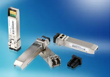
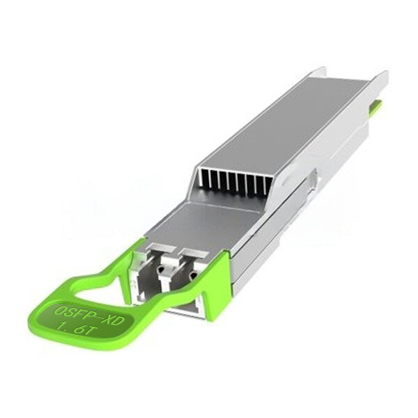
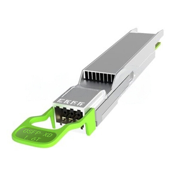
A 1.6T optical transceiver is the first module generation where the part number on the order form depends on the cooling in the rack row. Two years ago that sentence would have been an exaggeration. In 2026, it is a procurement reality.
Network engineers already know the arithmetic that got us here. GPU clusters outgrew 51.2T switch fabrics faster than the optics roadmap expected, and the spine that was comfortably 800G in 2024 became the bottleneck in 2026. What is harder to pin down is everything else: which form factor your switch cage actually accepts, which optical variant matches the fiber you already own, how many watts the row can dissipate, and whether the part will arrive before the GPUs do.
What Is a 1.6T Optical Transceiver?
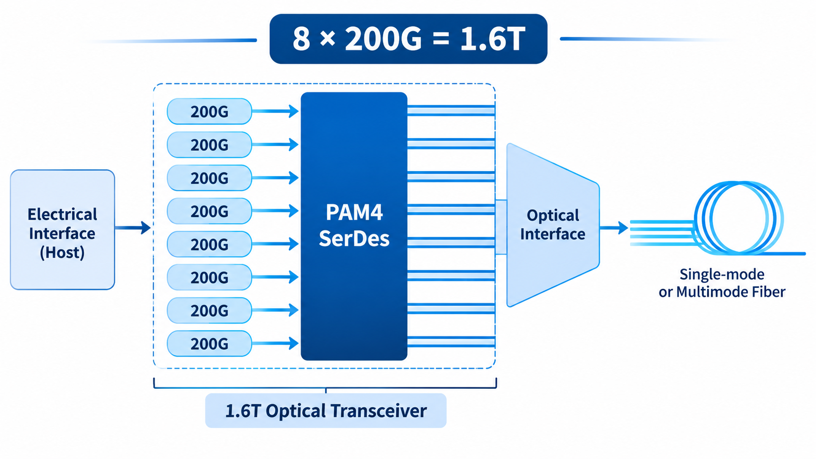
A 1.6T optical transceiver, also written as a 1600G optical transceiver, is an eight-lane pluggable module that carries 1,600 Gb/s of aggregate Ethernet traffic, using eight PAM4 lanes at roughly 200 Gb/s each. It sits in a switch or NIC cage like any other pluggable and transmits over single-mode fiber, multimode fiber, or copper cable depending on the variant.
The 1.6T optical module builds directly on the 800G generation. The lane count stays at eight. The per-lane data rate doubles. That single change drives every other difference in this article, from the baud rate to the connector count to the fault-finding procedure your field team will use.
A 1.6T optical transceiver typically uses eight optical lanes, each carrying approximately 200 Gb/s of Ethernet data. The 224G designation refers to the high-speed electrical signaling class rather than the actual Ethernet payload rate per optical lane. PAM4 modulation enables two bits per symbol, while the exact baud rate depends on the electrical and optical interface implementation.
Why 1.6T Arrived in 2026, Not Sooner
Three things had to line up, and all three landed in the same two-year window.
The switch silicon got there first. Broadcom’s Tomahawk 6 delivers 102.4 Tb/s of switching capacity in a single chip, packaged into systems that expose 64 × 1.6T ports. Edgecore’s AIS1600-64O, built on the Tomahawk 6C silicon, puts 64 OSFP1600 cages in a 2U chassis. Cisco’s Silicon One G300 and NVIDIA’s Spectrum-6 generation address the same capacity tier. A 102.4T switch with 800G optics needs 128 cages; with 1.6T optics it needs 64. Half the cages, half the modules, half the cable ends.
The standard caught up. IEEE P802.3dj reached conditional approval to forward to RevCom in October 2026, following a third Sponsor Ballot recirculation that closed at 97% approval. Publication is expected in December 2026. That timeline matters less than it sounds, because serious buyers have been deploying pre-standard parts for a year, but it removes the last procurement objection.
The optics supply chain matured, unevenly. 200G EML lasers moved from sampling to volume, and DSP vendors shipped 1.6T parts. Laser supply remains the tightest link in the chain, which is why lead times look the way they do.
The forecasts disagree, and that is informative
Ask five credible sources how many 1.6T modules will ship in 2026, and you will get numbers that differ by a factor of three.
| Source |
2026 1.6T shipment estimate |
| Cignal AI |
More than 10 million |
| ICC and research houses |
11 to 15 million |
| Citigroup |
About 22 million |
| TrendForce |
About 28 million |
| Goldman Sachs (raised Sept 2026) |
33 million, with 71 million for 2027 |
The spread is not sloppiness. The estimates differ because they count different things.
Some models only retimed DSP-based modules and exclude linear-drive parts. Some include twin-port 800G modules counted as 1.6T-equivalent ports. Some assume specific hyperscaler order books that are not public. And all of them have to guess how much 200G EML capacity will actually exist.
For planning purposes, treat the range as a range. What every source agrees on is direction: 1.6T shipments in 2026 are an order of magnitude above 2025, and the constraint is supply, not demand.
1.6T Form Factors: OSFP1600, OSFP-XD, QSFP-DD1600 and XPO
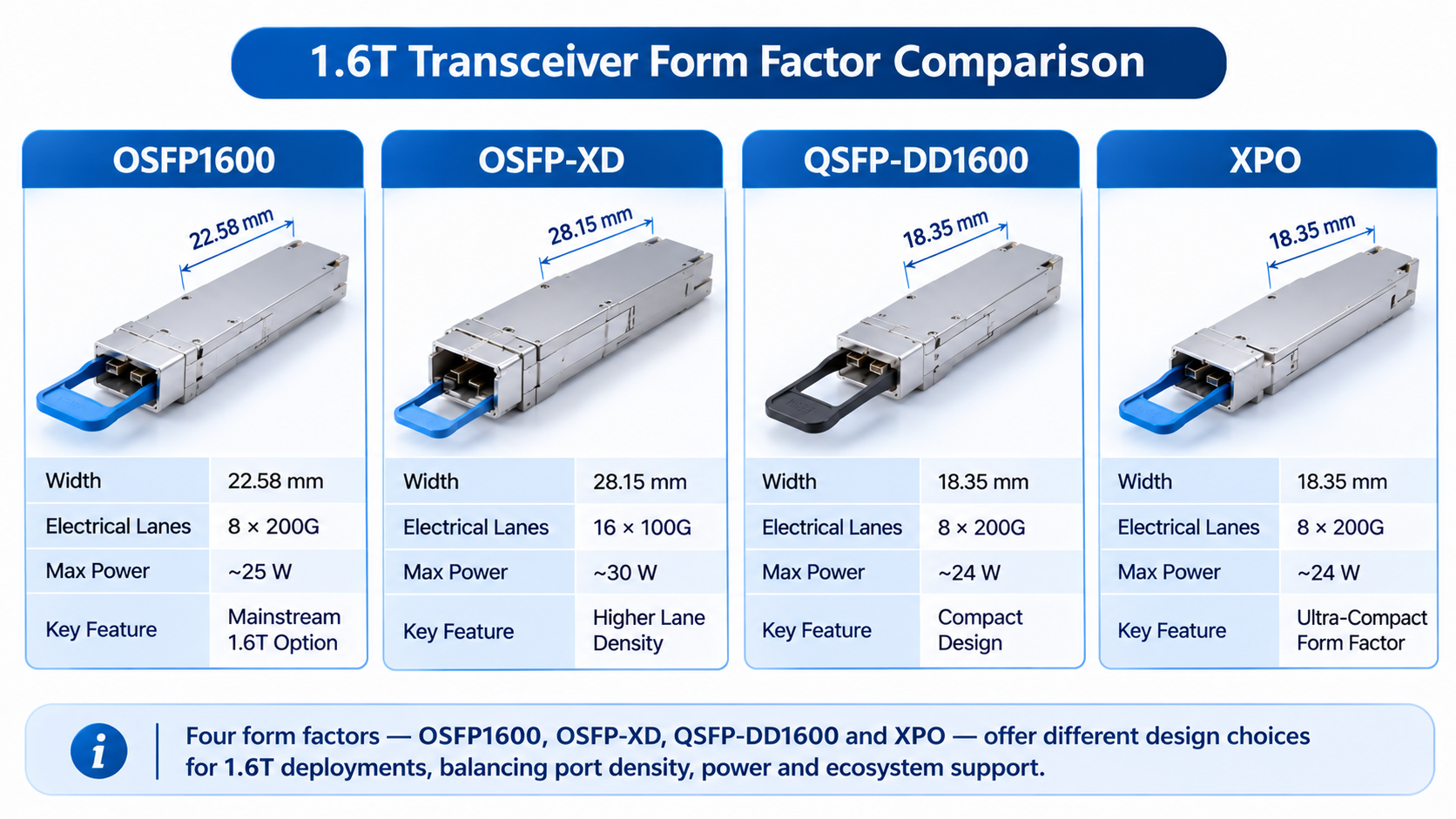
Four form factors carry 1.6T today, and they are not interchangeable. The table below is the complete comparison; each row links to deeper treatment where it exists.
| Form factor |
Electrical lanes |
Body width |
Cage compatibility |
Typical power |
Where it fits |
| OSFP1600 / OSFP224 |
8 × 200G |
22.58 mm |
1.6T-capable OSFP cage |
22 to 25 W |
The mainstream 2026 choice |
| OSFP-XD |
16 × 100G |
28.15 mm |
Requires an OSFP-XD cage |
Up to 33.5 W |
Earlier 1.6T route, narrower ecosystem |
| QSFP-DD1600 |
8 × 200G |
18.35 mm |
QSFP-DD cage, backward-compatible with QSFP-DD800, QSFP112 and QSFP56 |
25 to 30 W |
Density-first designs |
| XPO |
New multi-lane |
Larger |
New cage required |
Higher, liquid-cooled |
2027 and beyond |
An OSFP-XD module won’t seat in an OSFP cage, even though a standard OSFP module fits an OSFP-XD cage. The OSFP-XD body is 28.15 mm wide compared to 22.58 mm for OSFP, and the extra width carries eight additional electrical lanes. If your switch has OSFP cages, an OSFP-XD part is not an option.
The OSFP-XD path exists because it let vendors reach 1.6T with 100G-per-lane electrical signaling before 200G SerDes was ready. It shipped earlier, it works, and it carries a power penalty and a narrower interoperability story. For a full mechanical and electrical comparison, see our OSFP-XD vs OSFP analysis for 1.6T.
QSFP-DD1600 is the density play. At 18.35 mm wide, it fits 32 ports across a 1U faceplate where OSFP fits 24. Compatibility with lower-speed QSFP-family modules depends on the cage design, electrical interface, and host platform implementation. The catch is platform support. Juniper’s 1.6T documentation lists OSFP1600 only and explicitly excludes QSFP-DD1600, so confirm support per line card before specifying it.
For the mechanical details of OSFP itself, including the difference between flat-top and finned bodies, see the OSFP form factor guide and our OSFP 1.6T technical deep dive.
1.6T Optical Variants: DR8, DR8-2, 2×DR4 and 2×FR4
The variant determines your fiber, your connectors, and your link budget. There are four you will encounter in AI fabrics.
| Variant |
Reach |
Fibers |
Connector |
Link budget |
Typical power |
| 1.6T DR8 |
500 m |
16 SMF |
MPO-16 or 2 × MPO-12 APC |
3.0 dB |
22 W (23.8 W max) |
| 1.6T DR8-2 |
2 km |
16 SMF |
MPO-16 or 2 × MPO-12 APC |
4.0 dB |
23 to 25 W |
| 1.6T 2×DR4 |
500 m |
2 × 8 SMF |
2 × MPO-12 |
3.0 dB |
22 to 24 W |
| 1.6T 2×FR4 |
2 km |
4 SMF |
2 × duplex LC |
4.0 dB per link |
23.5 W (25 W max) |
The decision between them comes down to two questions. Do you have parallel fiber or duplex LC, and how much switch real estate can you spend on breakout?
DR8 is the parallel-fiber answer. Sixteen single-mode strands per link, MPO-16 or a pair of MPO-12 connectors, 500 m of reach with a 3.0 dB channel allowance. It is the natural spine-and-leaf interconnect inside a hall, and it is the variant most AI fabric designs standardize on.
DR8-2 extends the same 16-fiber plant to 2 km with a 4.0 dB budget, so campus or building-to-building runs above 500 m can keep existing MPO-12 trunking.
2×FR4 is the duplex-LC answer. It carries two independent 800G FR4 links in one housing, over four single-mode fibers and two duplex LC connectors, 2 km with a 4.0 dB budget per link. This is the variant that wins when the fiber plant already exists and re-pulling it is not on the table.
The reach wall is a margin wall
Here is the calculation that changes how people think about DR8.
A 500 m DR8 link has a 3.0 dB channel insertion-loss allowance. Take typical planning values: 0.47 dB per kilometer of single-mode fiber, 0.3 dB per splice, and 0.5 dB per mated connector pair. Four connector pairs at 0.5 dB plus the fiber gives 2.24 dB, leaving 0.76 dB of margin. Not generous, but workable.
Now substitute 0.75 dB per connector pair, which is realistic once you account for field-terminated ends, bulkhead adapters, and imperfect cleaning. Four pairs cost 3.0 dB on their own, plus the fiber loss, and you are over budget before a single splice. The link doesn’t fail because it is too long; it fails because the connectors used up the budget.
Two conclusions follow. Budget connector loss is 0.75 dB in design, not 0.5 dB. And the polish matters.
Connector endface types must match the transceiver specifications. APC and UPC connectors should never be directly mated, as their different endface geometries can cause excessive insertion loss and return loss.
Why there is no 1.6T LR8
Search for “1.6T LR8,” and you’ll find product pages. Search the standard and you won’t.
IEEE P802.3dj defines four port types for 1.6T: KR8 for backplanes, CR8 for copper cable, DR8 for 500 m single-mode, and DR8-2 for 2 km single-mode. This matters when you write a specification. For 10 km over duplex LC, a single-pluggable 1.6T answer doesn’t exist. Your options are 2 × 800G FR4, a 1.6T module plus external optics, or coherent 1.6T ZR at much higher cost and power. The 800G optical transceiver guide covers those fallbacks.
What Actually Changed at 200G Per Lane
The modulation scheme did not change. PAM4 with four amplitude levels still carries two bits per symbol. What changed is that the same scheme now runs at twice the symbol rate, roughly 106.25 GBd for DR8 and 113.4375 GBd for DR8-2 and 2×FR4.
That doubling compresses the engineering margin everywhere. Forward error correction is mandatory: RS(544,514) KP4, with an optional inner code in some implementations. Transmitter dispersion and eye closure penalty, TDECQ, is capped around 3.4 dB. A connector that contributed acceptable loss and reflection at 800G may now push the received signal below the FEC threshold.
The practical consequences show up in three places: connector hygiene, per-lane diagnostics, and the value of pre-deployment testing with the actual host. If you want the deeper theory, our PAM4 SerDes guide covers 200G-per-lane signaling.
Power, Heat and the Liquid-Cooling Decision
Power is where 1.6T stops being a connector decision and becomes an infrastructure decision.
| Architecture |
Module power |
Power per Tb/s |
| 800G DSP-based, twin-port OSFP |
15 to 17 W |
About 19 to 21 W/Tb/s |
| 1.6T DSP-based |
22 to 25 W |
About 14 to 16 W/Tb/s |
| 1.6T LRO (linear receive optics) |
About 16 W |
About 10 W/Tb/s |
| 1.6T LPO (linear pluggable optics) |
10 to 12 W |
About 6 to 8 W/Tb/s |
| Co-packaged or near-package optics |
About 9 W per port |
About 6 W/Tb/s |
The absolute wattage went up. The wattage per bit went down by roughly 25% against an 800G twin-port module, and by far more against 400G. That is the real economic argument for 1.6T in 2026, and it is stronger than the argument about sticker price.
Now scale it to a row. A fully populated 64-cage 1.6T switch draws around 1.5 kW through its optics alone, before the ASIC and the fans.
A 128-port 800G chassis draws roughly 1.9 to 2.2 kW at the same aggregate bandwidth. Same bandwidth, roughly 30% less optical power. That difference often decides whether a row can be air-cooled at all.
Finned or flat-top is an installation decision
OSFP modules come in two mechanical styles. The finned or riding heat sink version exposes fins above the cage and relies on chassis airflow. The flat-top or integrated heat sink version presents a flat surface for a cold plate or a direct-to-plug liquid loop.
Your platform decides this, not your preference. NVIDIA’s Quantum-X800 systems take twin-port OSFP modules in the integrated heat sink style, and ConnectX-8 adapters accept flat-top OSFP only. Specifying a finned module for a flat-top-only port produces a part that does not seat. The OSFP power consumption article covers the wattage ladder across body styles in more depth.
As module power approaches or exceeds 25 W, thermal management becomes increasingly challenging. Whether liquid cooling is required depends on the switch platform, airflow design, ambient temperature, and rack-level cooling capacity. Double-sided direct-to-plug cold plates are now shipping in 1.6T systems, and the 3.2T generation, expected around 50 W per module, will force liquid cooling on essentially every high-density port.
LPO and LRO at 1.6T
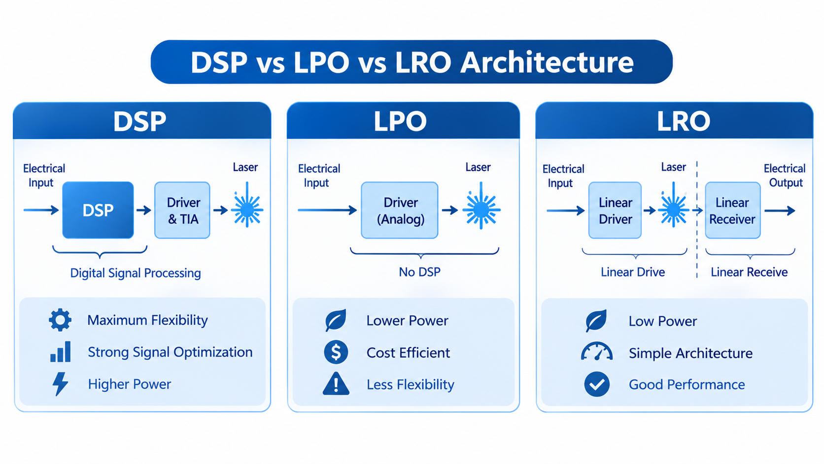
LPO can significantly reduce module power consumption by eliminating the DSP, although the actual savings depend on the optical architecture, host SerDes, and implementation.
The gate is host capability. LPO needs a host SerDes with enough linearity and a per-lane budget the module can meet, and not every 1.6T switch qualifies. Linear receive optics, or LRO, is the pragmatic middle path: transmit stays retimed, receive goes linear, and you recover a few watts without the full interoperability burden. LightCounting expects roughly 27% of 1.6T ports to use LPO by 2030.
If you are new to linear drive, the 800G LPO guide explains the fundamentals. At 1.6T, the physics are the same, and the margins are tighter.
Switch and NIC Compatibility
This is the section most 1.6T guides skip, and it is the one that decides whether your purchase order turns into working links.
| Platform |
Optics cages |
1.6T route |
Caveat |
| Broadcom Tomahawk 6 (102.4T) |
64 × 1.6T |
Native |
Cage population and body style depend on the system vendor |
| Edgecore AIS1600-64O (Tomahawk 6C) |
64 × OSFP1600 |
Native, 30 W per port |
Riding heat sink, front-to-back airflow |
| NVIDIA Spectrum-6 SN6810 (102.4T) |
128 × 800G |
Twin-port 800G or breakout |
Confirm the software release validates 1.6T twin-port optics |
| NVIDIA Quantum-X800 (115.2T) |
144 × 800G |
Twin-port 1.6T OSFP |
Integrated heat sink style only |
| NVIDIA ConnectX-8 |
Single-port 800G OSFP |
Not validated for 1.6T at the time of writing |
Flat-top OSFP only |
| Cisco Silicon One G300 |
64 × 1.6T class |
Native |
Line-card dependent |
| Juniper 1.6T platforms |
OSFP1600 only |
Native |
No QSFP-DD1600 support listed |
Three rules follow from that table.
“Compatible” and “supported” are different words. A module can meet every MSA and IEEE requirement and still not appear on a platform’s validated optics list. Firmware checks are real. NVIDIA’s ConnectX-8 release notes, for example, list validated cables and switches, and third-party 1.6T modules are not on that list at the time of writing. If your design depends on a specific NIC, verify against the release notes for the exact firmware version you will run.
Form factor compatibility is mechanical, not logical. A module that does not seat cannot be made to work with a software update. Check the cage, the body width, and the heat sink style before anything else.
Breakout changes the economics. A 1.6T OSFP twin-port module presenting 2 × 800G lets you connect to two 800G ports on an existing switch. That is how most organizations get 1.6T module density onto 800G-era fabrics during the transition. It also halves the effective port count per module, so do the fabric math before committing.
Our OSFP-compatible switches guide tracks platform support in more detail, and the OSFP-XD module guide covers the platform situation specific to that form factor.
1.6T in AI Fabrics: Port Counts and Attach Ratios
The reason 1.6T exists is that AI fabric bandwidth demand outran the port count available on switch silicon. The arithmetic is simple, and it explains everything about the economics.
A 102.4 Tb/s switch delivers 128 ports at 800G or 64 ports at 1.6T. Same bandwidth, half the ports. That halves the module count, the cage count, the cable ends, the connector cleaning labor, and the number of failure points in the fabric.
In a 512-GPU cluster, each GPU connects at 800G to a leaf switch, so the leaf tier alone carries 512 module ports before spine uplinks. Move the same cluster to 1.6T uplinks and the spine port count halves while its bandwidth stays constant.
The optics bill changes shape more than it changes size. A 1,024-GPU H200-class fabric costs roughly $3.5 million in optics at 800G and roughly $4.1 million at 1.6T, about a 17% capex premium, for roughly half the modules and a power per bit figure that improves from about 15 pJ/bit to about 9 pJ/bit. Whether that trade is worth it depends on whether your constraint is capital or power and rack space. In 2026, for most large clusters, it is power and rack space.
Cabling at 1.6T: DAC, ACC, AEC and AOC
Copper reach collapses at 200G per lane, and this surprises teams who are used to 800G copper.
| Cable type |
Practical reach at 1.6T |
| Passive DAC |
About 1 m |
| Active copper (ACC) |
About 2 m |
| Active electrical cable (AEC) |
3 to 5 m |
| Active optical cable (AOC) |
Tens of meters |
Compare that with 800G, where passive DAC commonly reaches 2.5 m, and AEC reaches 6.5 m. The 1.6T passive DAC is essentially a same-rack interconnect now. To connect a top-of-rack switch to a server two racks away, plan on AEC or AOC rather than copper.
Twin-port splitter cables matter here too. A 1.6T OSFP cage feeding two 800G QSFP-DD ports through a single passive cable is a legitimate brownfield bridge, and it is often the cheapest way to use 1.6T-capable switch ports while the server fleet is still 800G.
Migrating from 800G: A Phased Plan
Nobody replaces a working 800G fabric in one maintenance window, and the 800G vs 1.6T question is rarely all-or-nothing. The organizations doing this well run a four-phase plan.
Phase one: spine first. Upgrade the spine layer to 1.6T-capable switches while the leaves stay at 800G, connected through twin-port 1.6T modules. The spine is the bandwidth bottleneck in most AI fabrics, and it is the smallest layer to change.
Phase two: audit the fiber. Before buying anything, measure the plant. Connector polish, polarity, insertion loss, and return loss. A trunk that passes at 800G may fail the 3.0 dB DR8 budget at 1.6T, and finding that out after the modules arrive costs a quarter.
Phase three: leaves. Replace leaf optics as servers refresh. Keep an 800G spare pool sized for the transitional mix, not the target design.
Phase four: retire the bridge. Remove twin-port modules once every leaf port is native 1.6T.
Two constraints shape the schedule. Lead times for 1.6T modules run 12 to 24 weeks in 2026, against 2 to 8 weeks for 800G, where capacity is ample. And 200G EML supply is tight, with reported shortages anywhere from 20% to over 60% and DSP lead times exceeding a year.
An infrastructure team that locked a GPU delivery date before ordering optics ended up with racks powered and lit but unconnected for six weeks. Order optics before servers, not after.
When to stay on 800G
Honesty is worth more than a sales pitch here, so here is the case against 1.6T in 2026.
- Your fabric isn’t constrained. At 25.6T or 51.2T switch capacity, 1.6T ports mostly buy breakout complexity.
- Your power budget is fixed. Twenty-two-watt modules in 64 cages change a row’s thermal profile, and recooling the row isn’t in scope.
- Your lifecycle is standardized. Requalifying a new form factor can cost more than the bandwidth saves.
- Your volumes are small. The 1.6T premium per module is hardest to justify across a few dozen links.
1.6T earns its place at the spine of large accelerated clusters and in new builds where the cooling is designed for it. Everywhere else, 800G has another two years of good economics. The 400G-to-800G DR8 migration precedent shows how the last transition played out.
Price, Lead Time and Total Cost of Ownership
Published 1.6T module pricing in late 2026 clusters between $1,100 and $1,500, with a wider listing range from about $800 to $2,100 depending on variant, body style and quantity. An 800G module of comparable construction runs $350 to $450.
Per module, that is roughly a threefold premium. Per bit, it is much less dramatic.
| Module |
Price |
Cost per Gbps |
Cost per Tb/s |
| 800G DSP-based |
$400 |
$0.50 |
$500 |
| 1.6T DSP-based, low end |
$1,100 |
$0.69 |
$688 |
| 1.6T DSP-based, high-end |
$1,500 |
$0.94 |
$938 |
| 1.6T at parity with $400 800G |
$800 |
$0.50 |
$500 |
Parity arrives when a 1.6T module costs about $800 against a $400 800G module. Cost per Gbps has been declining roughly 20% a year, and the BOM gap is narrowing as 200G EML yields improve and silicon photonics variants reduce laser count.
The module price was never the decision. The normalization was.
Three cost factors are easy to miss.
DSP cost. The 1.6T DSP costs around $130 against $90 for 800G, and it is the largest single BOM line. It is also why LPO, which removes it, changes the cost curve.
Laser count and type. Eight 200G EMLs at roughly $160 each dominate an EML-based BOM. Silicon photonics and linear-drive designs reduce that.
Qualification and sparing. A new form factor needs new spare stock, new test fixtures, and new field training. Budget 10 to 15% of module spend for spares during the transition, not the 5% you carry in steady state.
Frequently Asked Questions
What is a 1.6T optical transceiver?
A 1.6T optical transceiver is an eight-lane pluggable module carrying 1,600 Gb/s of aggregate data, with each PAM4 lane running at about 200 Gb/s. It fits a switch or NIC cage and connects over single-mode fiber, multimode fiber, or copper depending on the variant.
How many lanes does a 1.6T transceiver have?
Eight optical lanes at 200 Gb/s each. OSFP-XD reaches 1.6T differently, using sixteen electrical lanes at 100 Gb/s, which is why it requires a wider body and a different cage.
What is the difference between 1.6T DR8 and DR8-2?
DR8 reaches 500 m over 16 single-mode fibers with a 3.0 dB link budget. DR8-2 reaches 2 km over the same fiber count with a 4.0 dB budget. Both use MPO-16 or dual MPO-12 connectors.
Is 1.6T Ethernet an approved standard?
IEEE P802.3dj received conditional approval to forward to RevCom in October 2026, following a third Sponsor Ballot recirculation at 97% approval. Publication is expected in December 2026. Deployment has been underway for a year on pre-standard parts.
Do 1.6T modules require liquid cooling?
Not always. Air cooling works up to about 25 W per port, which covers most DSP-based 1.6T modules in a well-designed row. Modules at the high end of the range, OSFP-XD parts approaching 33.5 W, and the coming 3.2T generation do require liquid cooling.
How much does a 1.6T optical module cost?
Published prices cluster between $1,100 and $1,500 per module in late 2026, against $350 to $450 for an 800G module. Normalized per Tb/s, that is roughly $690 to $940, compared with about $500 for 800G.
Can a 1.6T module run in an 800G OSFP cage?
Only if the cage is rated for 1.6T and the body style matches. An OSFP-XD module will not fit an OSFP cage at all. A 1.6T OSFP module needs a cage rated for its power and heat sink style, and the host firmware must validate it.
What is the lead time for 1.6T transceivers?
Twelve to 24 weeks in 2026, driven by 200G EML and DSP supply. Comparable 800G modules ship in 2 to 8 weeks. Order 1.6T optics well before the servers they connect.
Does 1.6T mean 224G per lane?
No. 224G describes the signaling class of the host electrical interface. The optical payload per lane is 200 Gb/s, at baud rates near 106.25 GBd or 113.4375 GBd depending on the variant.
Post Views: 148